Using Nested-Pandas with Astronomical Spectra#
In Astronomy, a spectrum is a measurement (or combination of measurements) of an object that shows the intensity of light emitted over a range of energies. In this tutorial, we’ll walk through a simple example of working with spectra from the Sloan Digital Sky Survey (SDSS), in particular showing how it can be represented as a NestedFrame.
First, we’ll use astroquery and astropy to download a handful of spectra from SDSS:
[3]:
from astroquery.sdss import SDSS
from astropy import coordinates as coords
import astropy.units as u
import nested_pandas as npd

# Query SDSS for a set of objects with spectra
pos = coords.SkyCoord("0h8m10.63s +14d50m23.3s", frame="icrs")
xid = SDSS.query_region(pos, radius=3 * u.arcmin, spectro=True)
xid_ndf = npd.NestedFrame(xid.to_pandas())
xid_ndf
[3]:
| ra | dec | objid | run | rerun | camcol | field | z | plate | mjd | fiberID | specobjid | run2d | |
|---|---|---|---|---|---|---|---|---|---|---|---|---|---|
| 0 | 2.076662 | 14.843455 | 1237652943176204410 | 1739 | 301 | 3 | 316 | -0.000464 | 6112 | 56191 | 560 | 6881654266119084032 | v5_13_2 |
| 1 | 2.023446 | 14.839824 | 1237652943176138868 | 1739 | 301 | 3 | 315 | 0.045591 | 751 | 52251 | 160 | 845594848269461504 | 26 |
| 2 | 2.016424 | 14.810989 | 1237652943176139005 | 1739 | 301 | 3 | 315 | 0.113535 | 752 | 52251 | 302 | 846759780839090176 | 26 |
3 rows × 13 columns
This initial query returns a set of objects with spectra (as specified by the spectro=True flag). To actually retrieve the spectra, we can do the following:
[4]:
# Query SDSS for the corresponding spectra
SDSS.clear_cache()
sp = SDSS.get_spectra(matches=xid)
sp
[4]:
[[<astropy.io.fits.hdu.image.PrimaryHDU object at 0x119f595e0>, <astropy.io.fits.hdu.table.BinTableHDU object at 0x11bc36600>, <astropy.io.fits.hdu.table.BinTableHDU object at 0x11bc74aa0>, <astropy.io.fits.hdu.table.BinTableHDU object at 0x11bc77d40>, <astropy.io.fits.hdu.table.BinTableHDU object at 0x11bc36e40>, <astropy.io.fits.hdu.table.BinTableHDU object at 0x11bc17320>, <astropy.io.fits.hdu.table.BinTableHDU object at 0x11bc92e70>, <astropy.io.fits.hdu.table.BinTableHDU object at 0x11bc938c0>, <astropy.io.fits.hdu.table.BinTableHDU object at 0x11bcbe1b0>, <astropy.io.fits.hdu.table.BinTableHDU object at 0x11bcd5d60>, <astropy.io.fits.hdu.table.BinTableHDU object at 0x11bce98e0>, <astropy.io.fits.hdu.table.BinTableHDU object at 0x11bd04650>],
 [<astropy.io.fits.hdu.image.PrimaryHDU object at 0x11bbbe090>, <astropy.io.fits.hdu.table.BinTableHDU object at 0x11bd06390>, <astropy.io.fits.hdu.table.BinTableHDU object at 0x11bd15b20>, <astropy.io.fits.hdu.table.BinTableHDU object at 0x11bd28ce0>, <astropy.io.fits.hdu.table.BinTableHDU object at 0x11bd2b320>, <astropy.io.fits.hdu.table.BinTableHDU object at 0x11bd424e0>, <astropy.io.fits.hdu.table.BinTableHDU object at 0x11bd51700>, <astropy.io.fits.hdu.table.BinTableHDU object at 0x11bd688f0>, <astropy.io.fits.hdu.table.BinTableHDU object at 0x11bd6bad0>, <astropy.io.fits.hdu.table.BinTableHDU object at 0x11bd7ecc0>],
 [<astropy.io.fits.hdu.image.PrimaryHDU object at 0x11bc34560>, <astropy.io.fits.hdu.table.BinTableHDU object at 0x11bd907a0>, <astropy.io.fits.hdu.table.BinTableHDU object at 0x11bda8080>, <astropy.io.fits.hdu.table.BinTableHDU object at 0x11bdab230>, <astropy.io.fits.hdu.table.BinTableHDU object at 0x11bdb9850>, <astropy.io.fits.hdu.table.BinTableHDU object at 0x11bdccaa0>, <astropy.io.fits.hdu.table.BinTableHDU object at 0x11bdcfcb0>, <astropy.io.fits.hdu.table.BinTableHDU object at 0x11bde6e40>, <astropy.io.fits.hdu.table.BinTableHDU object at 0x11bdf9fd0>, <astropy.io.fits.hdu.table.BinTableHDU object at 0x11be0d220>]]
The result is a list of FITS formatted data. From this point there are a few ways that we could move towards a nested-pandas representation. The most straightforward is to build a “flat” spectra table from all the objects, where we gather the information from each spectrum into a single combined table.
[5]:
import numpy as np

# Build a flat spectrum dataframe

# Initialize some empty arrays to hold the flat data
wave = np.array([])
flux = np.array([])
err = np.array([])
index = np.array([])
# Loop over each spectrum, adding its data to the arrays
for i, hdu in enumerate(sp):
    wave = np.append(wave, 10 ** hdu["COADD"].data.loglam)  # * u.angstrom
    flux = np.append(flux, hdu["COADD"].data.flux * 1e-17)  # * u.erg/u.second/u.centimeter**2/u.angstrom
    err = np.append(err, 1 / hdu["COADD"].data.ivar * 1e-17)  # * flux.unit

    # We'll need to set an index to keep track of which rows correspond
    # to which object
    index = np.append(index, i * np.ones(len(hdu["COADD"].data.loglam)))

# Build a NestedFrame from the arrays
flat_spec = npd.NestedFrame(dict(wave=wave, flux=flux, err=err), index=index.astype(np.int8))
flat_spec
/var/folders/lc/dws63_cs5gz5mf8s869hjpx40000gn/T/ipykernel_21256/2955152026.py:14: RuntimeWarning: divide by zero encountered in divide
  err = np.append(err, 1 / hdu["COADD"].data.ivar * 1e-17)  # * flux.unit
[5]:
| wave | flux | err | |
|---|---|---|---|
| 0 | 3606.617188 | 1.699629e-16 | 9.050196e-17 |
| 0 | 3607.447021 | -4.092098e-17 | 7.294453e-17 |
| ... | ... | ... | ... |
| 2 | 9185.439453 | 1.398144e-16 | 1.269789e-17 |
| 2 | 9187.557617 | 1.487952e-16 | 1.259023e-17 |
12245 rows × 3 columns
From here, we can simply nest our flat table within our original query result:
[ ]:
spec_ndf = xid_ndf.join_nested(flat_spec, "coadd_spectrum").set_index("objid")
spec_ndf
| ra | dec | run | rerun | camcol | field | z | plate | mjd | fiberID | specobjid | run2d | coadd_spectrum | ||||||||||
|---|---|---|---|---|---|---|---|---|---|---|---|---|---|---|---|---|---|---|---|---|---|---|
| 1237652943176204410 | 2.076662 | 14.843455 | 1739 | 301 | 3 | 316 | -0.000464 | 6112 | 56191 | 560 | 6881654266119084032 | v5_13_2 |
|
|||||||||
| 1237652943176138868 | 2.023446 | 14.839824 | 1739 | 301 | 3 | 315 | 0.045591 | 751 | 52251 | 160 | 845594848269461504 | 26 |
|
|||||||||
| 1237652943176139005 | 2.016424 | 14.810989 | 1739 | 301 | 3 | 315 | 0.113535 | 752 | 52251 | 302 | 846759780839090176 | 26 |
|
And we can see that each object now has the coadd_spectrum nested column with the full spectrum available.
[9]:
# Look at one of the spectra
spec_ndf.iloc[1].coadd_spectrum
[9]:
| wave | flux | err | |
|---|---|---|---|
| 0 | 3799.268555 | 3.059662e-16 | 1.552601e-16 |
| 1 | 3800.142578 | 3.324573e-16 | inf |
| ... | ... | ... | ... |
| 3839 | 9196.020508 | 5.023617e-16 | 3.563417e-17 |
| 3840 | 9198.140625 | 5.170272e-16 | 5.481493e-17 |
3841 rows × 3 columns
We now have our spectra nested, and can proceed to do any filtering and analysis as normal within nested-pandas.
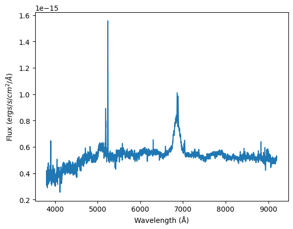
[10]:
import matplotlib.pyplot as plt

# Plot a spectrum
spec = spec_ndf.iloc[1].coadd_spectrum

plt.plot(spec["wave"], spec["flux"])
plt.xlabel("Wavelength (Å)")
plt.ylabel(r"Flux ($ergs/s/cm^2/Å$)")
[10]:
Text(0, 0.5, 'Flux ($ergs/s/cm^2/Å$)')